Airbnb Rome EDA

Introduction:

In this report we will be analyzing Rome Airbnb properties dataset from inside airbnb and try to analyze it to find what variables influences the income generted by the property.

Why Rome?

We choose Rome because it’s one of the most visited cities by tourists in Europe. Thanks to the rich history, amazing food, and the relatively cheaper prices compared to other major european cities. All of these factors make Rome one of the most sought after investments in the hospitality and tourism industry.

About the dataset source

We got our dataset from inside airbnb. Inside Airbnb is a project that provides data and advocacy about Airbnb’s impact on residential communities. They provide data and information to empower communities to understand, decide and control the role of renting residential homes to tourists.

Data dictionary

Variable	Description
host_name	Name of the host.
neighbourhood	Name of the neighbourhood.
latitude	Used to make an interactive map.
longitude	Used to make an interactive map.
room_type	Entire apt, private room, hotel room.
Price	Price in Euro.
minimum_nights	minimum number of night stay for the listing.
number_of_reviews	The number of reviews the listing has.
last_review	The date of the last/newest review.
availability_365	The availability of the listing x days in the future.
number_of_reviews_ltm	The number of reviews the listing has (in the last 12 months).
amenities	A list of amenities in the listing.

Data Munging

First we will be doing basic data cleaning

Importing libraries and Data

Code

import pandas as pd
import numpy as np
import matplotlib.pyplot as plt
import seaborn as sns
import plotly.express as px
import plotly.graph_objects as go
import folium
from folium.plugins import MarkerCluster
from folium import plugins
from folium.plugins import FastMarkerCluster
from folium.plugins import HeatMap
from ast import literal_eval
from plotly.subplots import make_subplots


df = pd.read_csv('data/listings.csv')
df2 = pd.read_csv('data/listings-detailed.csv')

df.head(5)

	id	name	host_id	host_name	neighbourhood_group	neighbourhood	latitude	longitude	room_type	price	minimum_nights	number_of_reviews	last_review	reviews_per_month	calculated_host_listings_count	availability_365	number_of_reviews_ltm	license
0	49955080	Singola al Casale di Gardenia	396326393	Alessia	NaN	XV Cassia/Flaminia	42.07605	12.32067	Private room	66	1	0	NaN	NaN	3	88	0	NaN
1	41146116	Il Giardino di Veio	322089651	Rosetta	NaN	XV Cassia/Flaminia	42.05088	12.45619	Private room	20	2	1	2020-01-26	0.03	1	0	0	NaN
2	39624404	CAMERA MATRIMONIALE STANDARD CON COLAZIONE INC...	304471512	Hotel	NaN	VI Roma delle Torri	41.82882	12.73900	Private room	100	1	0	NaN	NaN	1	180	0	NaN
3	1903817	Lovely apartment with fabulous view north of Rome	9883614	Eva	NaN	XV Cassia/Flaminia	42.13578	12.32621	Entire home/apt	110	3	53	2022-05-25	0.63	4	289	3	NaN
4	17617868	SUPER OFFERTA-stanza Maria-doppia o matrimoniale	97622372	Eleonora	NaN	XV Cassia/Flaminia	42.06512	12.46106	Private room	25	1	12	2022-05-17	0.19	3	315	3	16903

Cleaning Data

First we checked for duplicates and null values

Code

df.duplicated().sum()

df.isnull().sum()

id                                    0
name                                  3
host_id                               0
host_name                             5
neighbourhood_group               23911
neighbourhood                         0
latitude                              0
longitude                             0
room_type                             0
price                                 0
minimum_nights                        0
number_of_reviews                     0
last_review                        3941
reviews_per_month                  3941
calculated_host_listings_count        0
availability_365                      0
number_of_reviews_ltm                 0
license                           20387
dtype: int64

there was no duplicates but we have null values in host_id, host_name, neighbourhood_group, licence and . We decided to drop the missing values for all columns except reviews.

Second we used apply to convert the price in the dataset to float. We also decided to drop price values of 0 and bigger than 50000 as there was nothing interesting to investigate there and they will miss up our result.

Code

df2["price"]=df2["price"].apply(lambda x : float(x[1:].replace(",","")))
df2.drop(df2[df2["price"]>=50000].index,axis=0,inplace=True)
df2.drop(df2[df2["price"]==0].index,axis=0,inplace=True)

The amenities column has amenities written as a list inside a string, so we will use literal_eval from ast to turn it into lists of strings, then use explode from pandas to give each element of the list it’s own row, and lastly we will perform a one hot encoding using crosstab

Code

df2["amenities"] = df2["amenities"].apply(literal_eval)
exploded_df2 = df2.explode('amenities')
df_new = pd.crosstab(exploded_df2['id'],exploded_df2['amenities']).rename_axis(None,axis=1).add_prefix("amenities_")

Code

df = pd.concat([df.set_index("id"), df_new], axis=1, join='inner').reset_index()
df = df.join(df2[["review_scores_rating", "review_scores_accuracy", "review_scores_cleanliness", "review_scores_checkin", "review_scores_communication", "review_scores_location", "review_scores_value"]])

EDA

Listings by neighbourhood

Here we want to see how many listings we have per neighbourhood

Code

dist_plt = df['neighbourhood'].value_counts().nlargest(5).plot.bar()
plt.xticks(rotation = 30)

(array([0, 1, 2, 3, 4]),
 [Text(0, 0, 'I Centro Storico'),
  Text(1, 0, 'VII San Giovanni/Cinecittà'),
  Text(2, 0, 'II Parioli/Nomentano'),
  Text(3, 0, 'XIII Aurelia'),
  Text(4, 0, 'XII Monte Verde')])

We can see from this fig above that most of the listings in our dataset are located at I Centro Storico.

Now lets see how these listing appear on a map using folium library

Code

Long=12.6
Lat=41.8
locations = list(zip(df.latitude, df.longitude))

map1 = folium.Map(location=[Lat,Long], zoom_start=10.5)
FastMarkerCluster(data=locations).add_to(map1)
map1

Make this Notebook Trusted to load map: File -> Trust Notebook

As we can see, most of the listings are located in the city center.

Next we want to see the distribution of listings type in the dataset

Code

df['room_type'].value_counts().plot(kind = 'bar', color = ['g', 'r', 'b', 'y'])
plt.title('Listings type count')
plt.xticks(rotation = 30)

(array([0, 1, 2, 3]),
 [Text(0, 0, 'Entire home/apt'),
  Text(1, 0, 'Private room'),
  Text(2, 0, 'Hotel room'),
  Text(3, 0, 'Shared room')])

The plot above shows us that most listings are of type Entire Apt, followed by Private room and Hotel room.

Lets also see what’s the median price per neighbourhood

Code

mode_dist_plt = df.groupby('neighbourhood')['price'].median().nlargest(5).plot.bar()
plt.title('Median price per neighbourhood (Top 5)')
plt.xticks(rotation = 30)

(array([0, 1, 2, 3, 4]),
 [Text(0, 0, 'I Centro Storico'),
  Text(1, 0, 'XIII Aurelia'),
  Text(2, 0, 'XV Cassia/Flaminia'),
  Text(3, 0, 'II Parioli/Nomentano'),
  Text(4, 0, 'XII Monte Verde')])

The highest median price is in I Centro Storico, followed by XIII Aurelia.

Now lets check for mean price per neighbourhood

Code

mean_dist_plt = df.groupby('neighbourhood')['price'].mean().nlargest(5).plot.bar()
plt.title('Mean price per neighbourhood (Top 5)')
plt.xticks(rotation = 30)

(array([0, 1, 2, 3, 4]),
 [Text(0, 0, 'I Centro Storico'),
  Text(1, 0, 'II Parioli/Nomentano'),
  Text(2, 0, 'XIII Aurelia'),
  Text(3, 0, 'XV Cassia/Flaminia'),
  Text(4, 0, 'IX Eur')])

The highest mean price is in XIII Aurelia, followed by I Centro Storico.

Let’s also look at the heatmap of the listings above 300 euro

Code

df_50 = df[df['price']>=300]


map2=folium.Map([42,12],zoom_start=9.8)
location = ['latitude','longitude']
df_map = df_50[location]
HeatMap(df_map.dropna(),radius=8,gradient={.4: 'blue', .65: 'lime', 1: 'red'}).add_to(map2)
map2

Make this Notebook Trusted to load map: File -> Trust Notebook

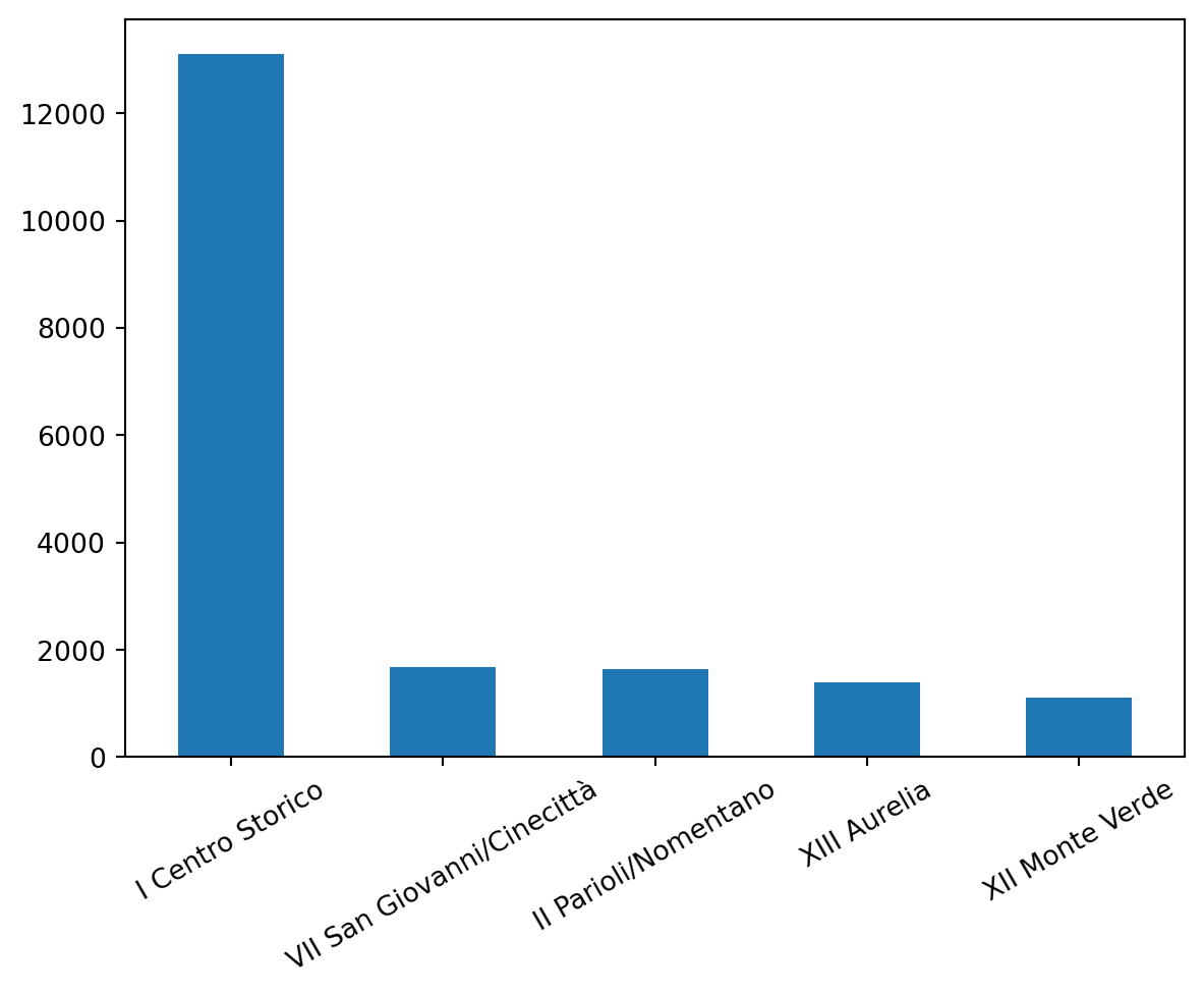
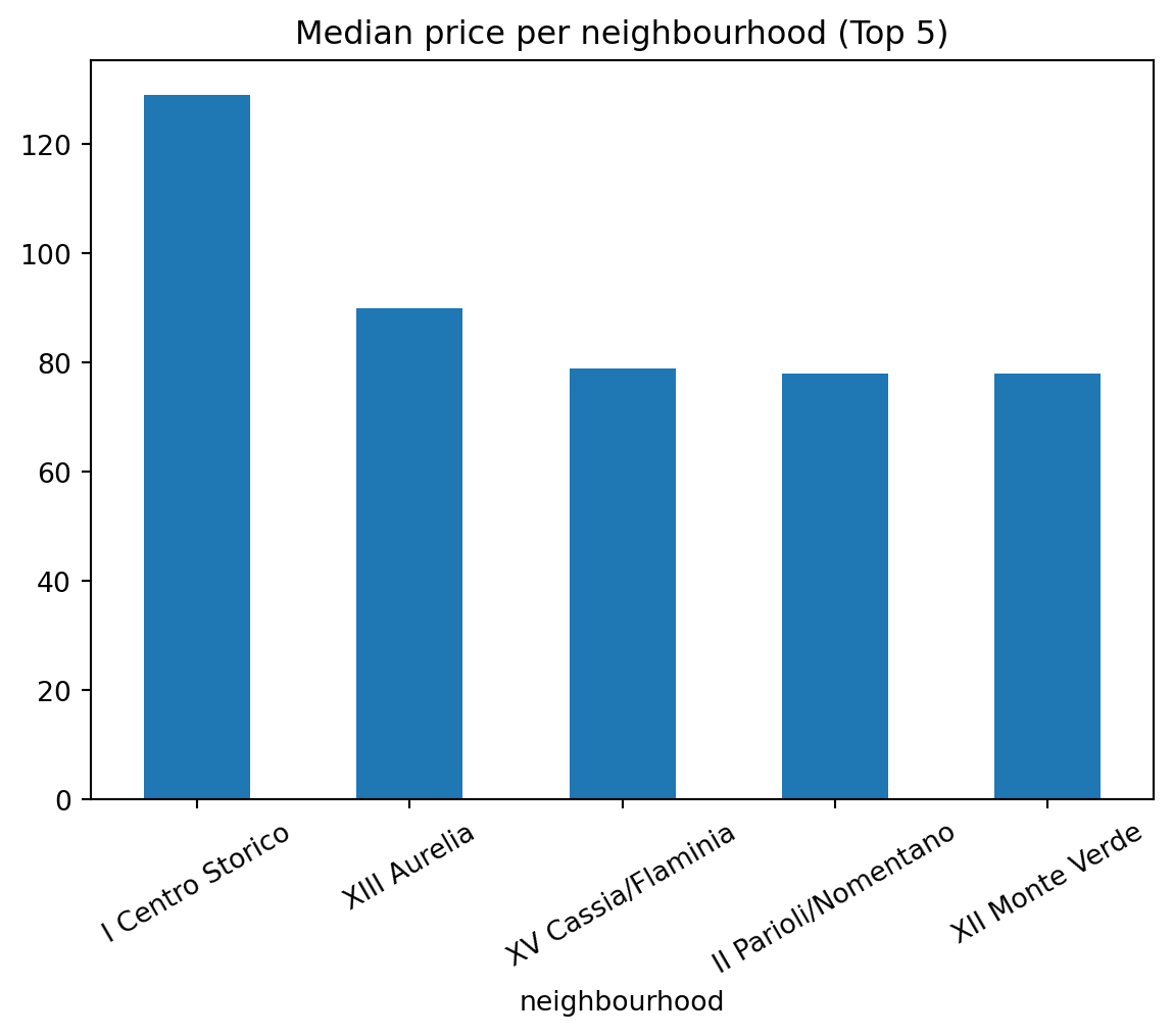
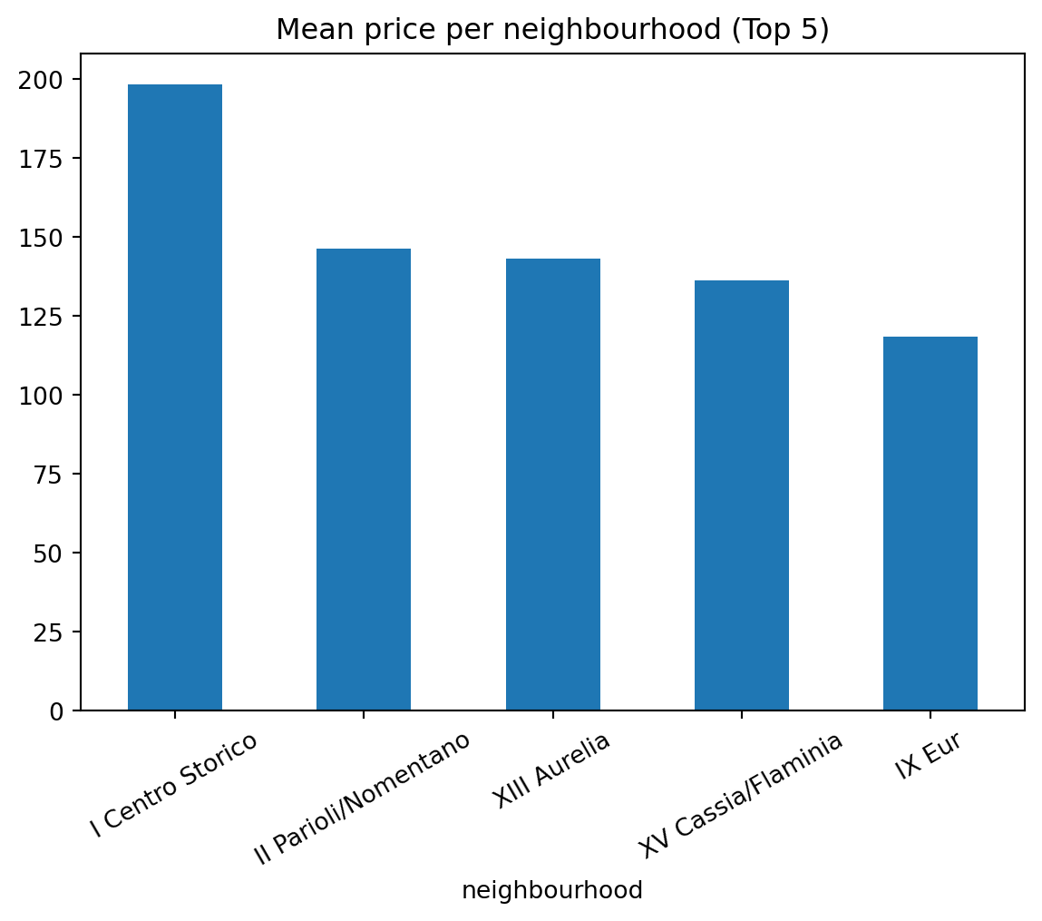
We also see here that the highest prices are in I Centro Storico.

Amenities and Price

What are the most frequent amenities in Roma listings?

Code

amenities = {}
for c in df.columns:
    if "amenities" in c: 
        amenities[c] = df[c].value_counts()[1]
amenities_list = sorted(amenities, key=amenities.get, reverse=True)[:10]
amenities = {c:df[c].value_counts()[1] for c in amenities_list}
fig = px.bar(x = amenities.keys(), y = amenities.values(), title = "Most Frequent Amenities", labels={
    "y": "Count",
    "x": "Amenities"
})
fig.show()

We can see that Wifi is the most frequent amenity in Roma’s listings, followed bt Essentials, Hair dryer, and Long term stay. This amenities might be the basic or standard amenities that a vistor to Roma would want.

What is the average price for the most frequent Amenities?

Code

amenities = {}
for c in df.columns:
    if "amenities" in c: 
        amenities[c] = df[c].value_counts()[1]
amenities_list = sorted(amenities, key=amenities.get, reverse=True)[:10]
amenities = {c:df.groupby(c)['price'].mean()[1] for c in amenities_list}
fig = px.bar(x = amenities.keys(), y = amenities.values(), title = "Average Price for the Most Frequent Amenities", labels={
    "y": "Average Price",
    "x": "Amenities"
})
fig.show()

from the above graph we can see that listsings that have Air Conditioning, have the highest average price with 185.24

What are the most expensive Amenities?

Code

amenities = {}

for c in df.columns:
    if "amenities" in c: 
        amenities[c] = df.groupby(c)['price'].mean()[1]

amenities_list = sorted(amenities, key=amenities.get, reverse=True)[:10]
amenities = {c:df.groupby(c)['price'].mean()[1] for c in amenities_list}
amenities_count = {c:df[c].value_counts()[1] for c in amenities_list}

fig = px.bar(x = amenities.keys(), y = amenities.values(), title = "Average Price for the Most Expnsive Amenities", labels={
    "y": "Average Price",
    "x": "Amenities"
})

fig.show()

The most expensive listings amenity is Outdoor seating with a 10.5K, followed by Piastre electric stove, Balcony, and Security cameras.

What is the distribution of the most expensive Amenities?

Code

amenities = {}

for c in df.columns:
    if "amenities" in c: 
        amenities[c] = df.groupby(c)['price'].mean()[1]

amenities_list = sorted(amenities, key=amenities.get, reverse=True)[:10]
amenities_count = {c:df[c].value_counts()[1] for c in amenities_list}

fig = px.bar(x = amenities_count.keys(), y = amenities_count.values(), title = "The Distribution of the Most Expnsive Amenities", labels={
    "y": "Count",
    "x": "Amenities"
})

fig.show()

We can see that only one listing has an outdoor seating and Piastre electric stove, while three listings have Balcony and two lsitings have security camera, although these amenities are in expensive listings they seems not to be frequent in Roma.

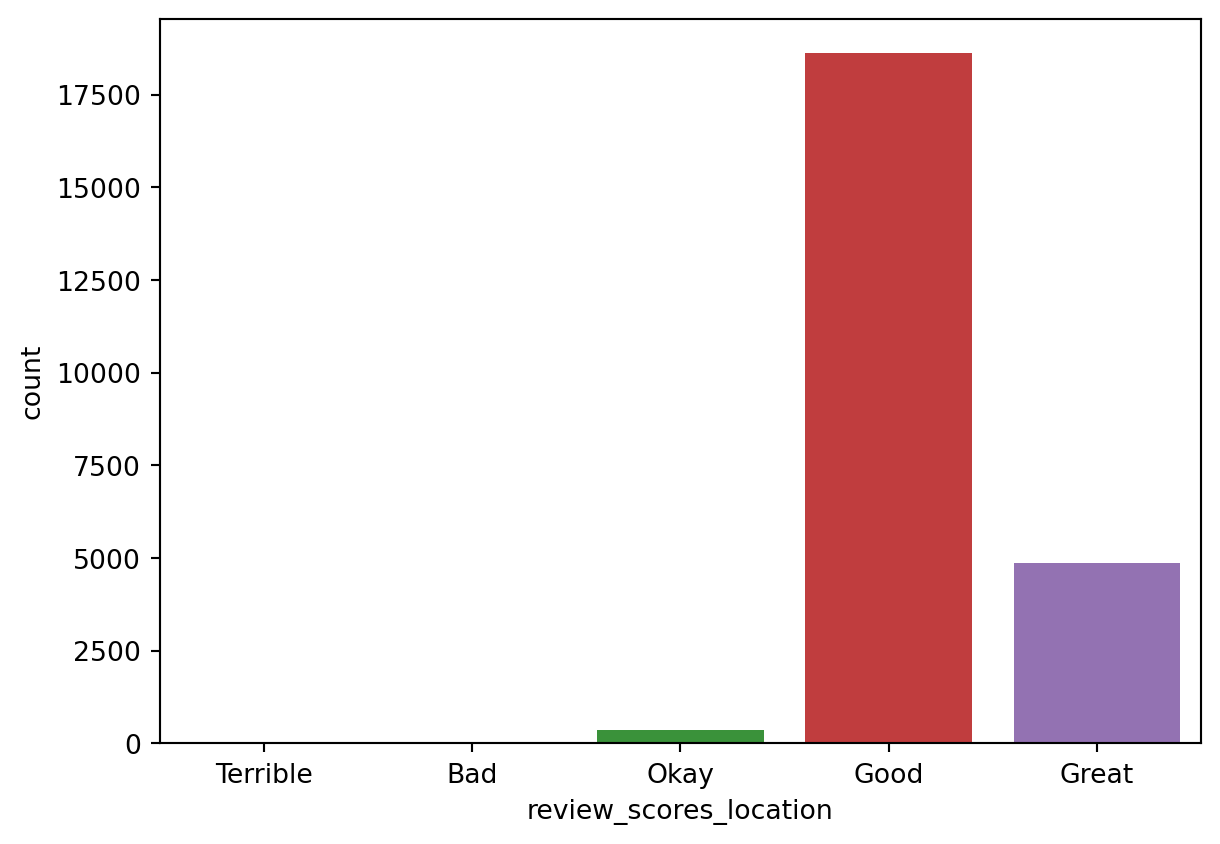
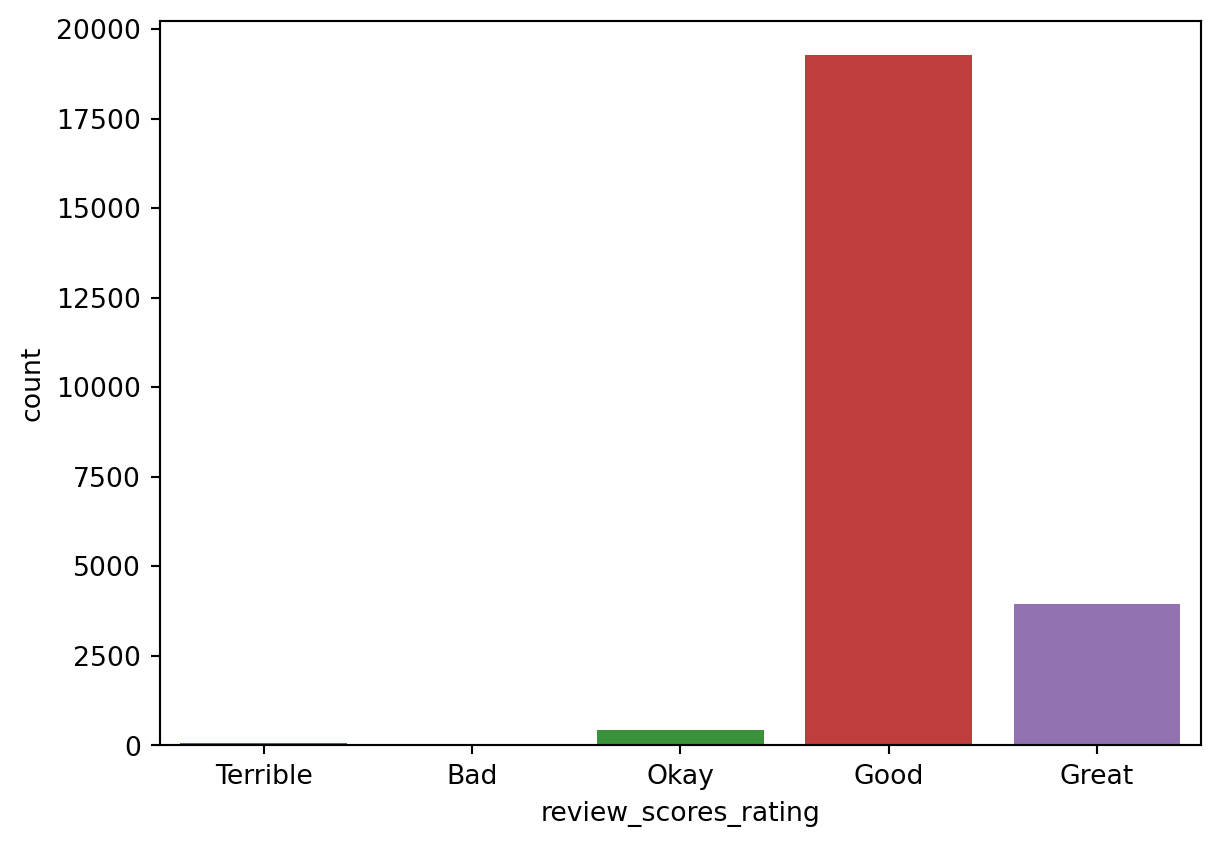
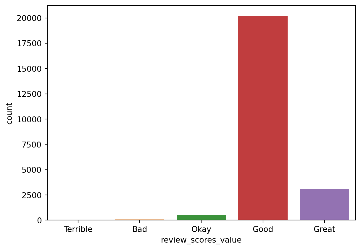
Distribution of Review’s Rating Scores

Code

for c in df.columns:
    if "scores" in c:
        df[c].fillna(df[c].mean(), inplace=True)

Code

rating_location_category = pd.cut(df.review_scores_location,bins=[1, 2, 3, 4, 5, 6], labels=["Terrible","Bad","Okay","Good", "Great"], right=False)
df['rating_location_category'] = rating_location_category
sns.countplot(x = rating_location_category)

<AxesSubplot:xlabel='review_scores_location', ylabel='count'>

Code

rating_category = pd.cut(df.review_scores_rating,bins=[1, 2, 3, 4, 5, 6],labels=["Terrible","Bad","Okay","Good", "Great"], right=False)
df['rating_category'] = rating_category
sns.countplot(x = rating_category)

<AxesSubplot:xlabel='review_scores_rating', ylabel='count'>

Code

value_category = pd.cut(df.review_scores_value,bins=[1, 2, 3, 4, 5, 6],labels=["Terrible","Bad","Okay","Good", "Great"], right=False)
df['value_category'] = value_category
sns.countplot(x = value_category, data=df)

<AxesSubplot:xlabel='review_scores_value', ylabel='count'>

It seems that in all three types of review’s scores,Good is the most frequent one followed by

Does the rating score effect the price

Code

data = df.groupby("rating_category")["price"].mean()
sns.barplot(x=data.index, y=data)

<AxesSubplot:xlabel='rating_category', ylabel='price'>

It seems that there is no relation between review_scores_rating and price.

what is the income of the past year and the expected income for the next 3 months?

• More data cleaning

Code

romeListings = df2.copy()
romeListings.at[19678,"minimum_minimum_nights"]=7
romeListings.drop(14443,inplace=True)
romeListings.drop(7022,inplace=True)
romeListings.at[5888,"minimum_minimum_nights"]=3
romeListings.drop(7250,inplace=True)
romeListings.at[11454,"minimum_minimum_nights"]=5
romeListings.at[20421,"price"]=121.51
romeListings.at[23230,"price"]=90
romeListings.at[9646,"price"]=92.73
romeListings.at[4737,"minimum_minimum_nights"]=3
romeListings.drop(romeListings[romeListings["price"]==0].index,inplace=True)

• add min_booked_nights_past_12m and min_income_past_12m column to the dataset

Code

#the minimum estmtation of the number of booked nights of each listing in the last 12 month (current date = 2022-06-07)
romeListings["min_booked_nights_past_12m"]=romeListings.apply(lambda x : x["number_of_reviews_ltm"]*x["minimum_nights_avg_ntm"],axis=1)

#the minimum estmtation of the income of each listing in the last 12 month (current date = 2022-06-07)
romeListings["min_income_past_12m"]=romeListings.apply(lambda x : x["min_booked_nights_past_12m"]*x["price"],axis=1)

• add expected_booked_nights_coming_3m and expected_income_coming_3m column to the dataset

Code

#the expected number of booked nights of each listing in the next 3 month (current date = 2022-06-07)
romeListings["expected_booked_nights_coming_3m"]=romeListings.apply(lambda x : 90-x["availability_90"],axis=1)

#the expected income of each listing  in the next 3 month (current date = 2022-06-07)
romeListings["expected_income_coming_3m"]=romeListings.apply(lambda x : (90-x["availability_90"])*x["price"],axis=1)

what neighbourhoods have highest averege price ?

Code

temp=romeListings.groupby("neighbourhood_cleansed")["price"].mean().sort_values(ascending=False).head(5).reset_index()
fig = px.bar(temp,x = "neighbourhood_cleansed", y = "price", title = "The highest price per night average of listings within a neighbourhood",color="neighbourhood_cleansed", labels={
    "y": "Price",
    "x": "Neighbourhood"
})
fig.show()

what neighbourhoods have highest averege of booked nights over the next 3 month ?

Code

temp=romeListings.groupby("neighbourhood_cleansed")["expected_booked_nights_coming_3m"].mean().sort_values(ascending=False).head(50).reset_index()
fig = px.bar(temp,x = "neighbourhood_cleansed", y = "expected_booked_nights_coming_3m", title = "The highest booked nights average of listings within a neighbourhood",color="neighbourhood_cleansed", labels={
    "y": "Booked nights (next 3 months)",
    "x": "Neighbourhood"
},range_y=[0,90])
fig.show()

what room types have highest averege price ?

Code

temp=romeListings.groupby("room_type")["price"].mean().sort_values(ascending=False).head(5).reset_index()
fig = px.bar(temp,x = "room_type", y = "price", title = "The highest price per night average of listings of a room type  ",color="room_type", labels={
    "y": "Price",
    "x": "Room Type"
})
fig.show()

what room types have highest averege of booked nights over the next 3 month ?

Code

temp=romeListings.groupby("room_type")["expected_booked_nights_coming_3m"].mean().sort_values(ascending=False).reset_index()
fig = px.bar(temp,x = 'room_type', y = "expected_booked_nights_coming_3m", title = "The highest booked nights average of listings of a room type",color="room_type", labels={
    "y": "Booked nights (next 3 months)",
    "x": "Room Type"
},range_y=[0,90])
fig.show()

what (room type ,neighbourhood) combinations have the highest averege booked nights ?

Code

nBookedNightinNigh=romeListings.groupby(["room_type","neighbourhood_cleansed"])["expected_booked_nights_coming_3m"].agg(["mean","count"])
temp=nBookedNightinNigh[nBookedNightinNigh["count"]>11]["mean"].sort_values(ascending=False).head(5)
fig = px.bar(x = list(map(str,list(temp.keys()))), y = temp.values, title = "The highest booked nights average of listings for every (Room Type,Neighbourhood) combination", labels={
    "y": "Booked nights (next 3 months)",
    "x": "(Room Type,Neighbourhood)"
},range_y=[0,90])
fig.show()

what neighbourhoods have highest minumam income average for the past 12 months ?

Code

temp=romeListings.groupby("neighbourhood_cleansed")["min_income_past_12m"].mean().sort_values(ascending=False).head(5).reset_index()
fig = px.bar(temp,x = "neighbourhood_cleansed", y = "min_income_past_12m", title = "The highest minimum income of listings within a Neighbourhood",color="neighbourhood_cleansed", labels={
    "y": "average minimum income of listings (past 12 months)",
    "x": "Neighbourhood"
})

fig.show()

what neighbourhoods with the highest expected income average for the next 3 months ?

Code

temp= romeListings.groupby("neighbourhood_cleansed")["expected_income_coming_3m"].mean().sort_values(ascending=False).head(5).reset_index()
fig = px.bar(temp,x = "neighbourhood_cleansed", y = "expected_income_coming_3m", title = "The highest expected income of listings within a Neighbourhood",color="neighbourhood_cleansed", labels={
    "y": "average expected income of listings (next 3 months)",
    "x": "Neighbourhood"
})

fig.show()

what room types have highest minumam income average for the past 12 months ?

Code

temp=romeListings.groupby("room_type")["min_income_past_12m"].mean().sort_values(ascending=False).head(5).reset_index()
fig = px.bar(temp,x = "room_type", y = "min_income_past_12m", title = "The highest minimum income of listings based on room type",color="room_type", labels={
    "y": "average minimum income of listings (past 12 months)",
    "x": "Room Type"
})

fig.show()

what room types have highest expected income average for the next 3 months ?

Code

temp=romeListings.groupby("room_type")["expected_income_coming_3m"].mean().sort_values(ascending=False).head(5).reset_index()
fig = px.bar(temp,x = "room_type", y = "expected_income_coming_3m", title = "The highest expected income of listings based on room type",color="room_type", labels={
    "y": "average expected income of listings (next 3 months)",
    "x": "Room Type"
})

fig.show()

what (room type ,neighbourhood) combinations have the highest averege income ?

Code

nBookedNightinNigh=romeListings.groupby(["room_type","neighbourhood_cleansed"])["expected_income_coming_3m"].agg(["mean","count"])
temp=nBookedNightinNigh[nBookedNightinNigh["count"]>11]["mean"].sort_values(ascending=False).head(5)
fig = px.bar(x = list(map(str,list(temp.keys()))), y = temp.values, title = "The highest income average of listings for every (Room Type,Neighbourhood) combination", labels={
    "y": "average income (next 3 months)",
    "x": "(Room Type,Neighbourhood)"
},)
fig.show()

does the host’s account appearance effects the listing income ?

Code

temp=romeListings.groupby("host_has_profile_pic")["expected_income_coming_3m"].mean().reset_index()
fig = px.bar(temp,x = ["No","Yes"], y = "expected_income_coming_3m", title = "",color=["No","Yes"], labels={
    "y": "average income (next 3 months)",
    "x": "host has a profile pic ?"
})
fig.show()

Code

temp= romeListings.groupby("host_identity_verified")["expected_income_coming_3m"].mean().reset_index()
fig = px.bar(temp,x = ["No","Yes"], y = "expected_income_coming_3m", title = "",color=["No","Yes"], labels={
    "y": "average income (next 3 months)",
    "x": "is the host identity verified ?"
},)
fig.show()

Code

temp= romeListings.groupby("instant_bookable")["expected_income_coming_3m"].mean()
fig = px.bar(temp,x = ["No","Yes"], y = "expected_income_coming_3m", title = "",color=["No","Yes"], labels={
    "y": "average income (next 3 months)",
    "x": "can be booked instantly ?"
},)
fig.show()

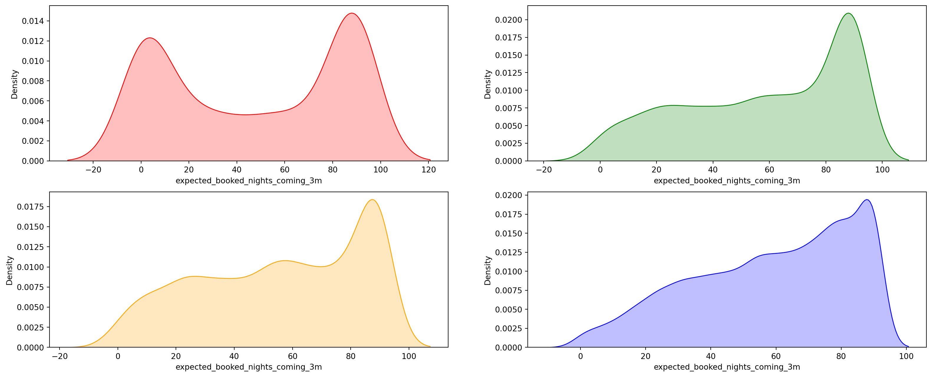
does the response time effects the the densisty of the number of the booked nights ?

Code

f, axes = plt.subplots(2, 2, figsize=(20,8))
ax = sns.kdeplot(romeListings[romeListings["host_response_time"]=="a few days or more"]["expected_booked_nights_coming_3m"],x="expected_booked_nights_coming_3m",color="red", fill=True,ax=axes[0,0])
ax = sns.kdeplot(romeListings[romeListings["host_response_time"]=="within a day"]["expected_booked_nights_coming_3m"],x="expected_booked_nights_coming_3m",color="green", fill=True,ax=axes[0,1])
ax = sns.kdeplot(romeListings[romeListings["host_response_time"]=="within a few hours"]["expected_booked_nights_coming_3m"],x="expected_booked_nights_coming_3m",color="orange",  fill=True,ax=axes[1,0])
ax = sns.kdeplot(romeListings[romeListings["host_response_time"]=="within an hour"]["expected_booked_nights_coming_3m"],x="expected_booked_nights_coming_3m",color="blue",  fill=True,ax=axes[1,1])

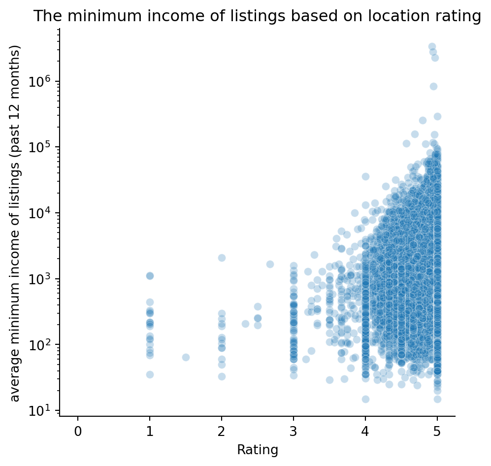
Does the Location Rating effect the minimum income of listings (past 12 months)

Code

romeListings[["rating_location_category", "rating_category", "value_category"]] = df[["rating_location_category", "rating_category", "value_category"]]

ax = sns.relplot(data= romeListings, x="review_scores_location", y ="min_income_past_12m" ,alpha=0.25)
plt.xticks([0, 1, 2, 3, 4, 5], ["0", "1", "2", "3", "4", "5"])
plt.yscale("log")
plt.title("The minimum income of listings based on location rating")
plt.xlabel("Rating")
plt.ylabel("average minimum income of listings (past 12 months)")
plt.show()

We can see that there is an upward trend that indicate, that listings with higher location review score had higher average minimum income for the past year.

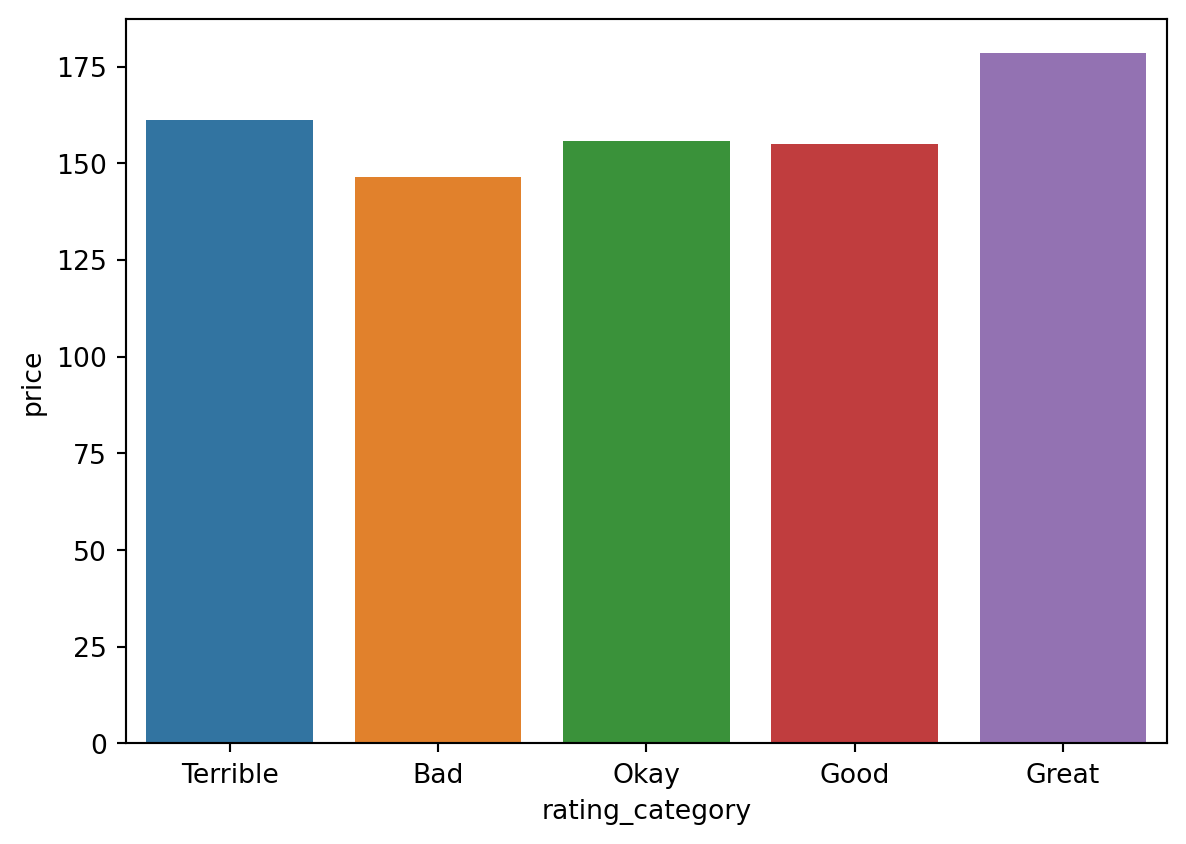
Code

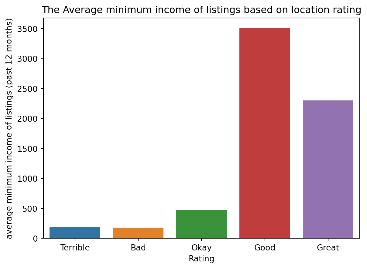
data = romeListings.groupby("rating_location_category")["min_income_past_12m"].mean().sort_values(ascending=False)
sns.barplot(x=data.index, y=data)
plt.title("The Average minimum income of listings based on location rating")
plt.xlabel("Rating")
plt.ylabel("average minimum income of listings (past 12 months)")
plt.show()

We can see here also that Good and Great, both have higher average minimum income than the rest of the categories.

What about the expected income for the next 3 months? let’s check it out.

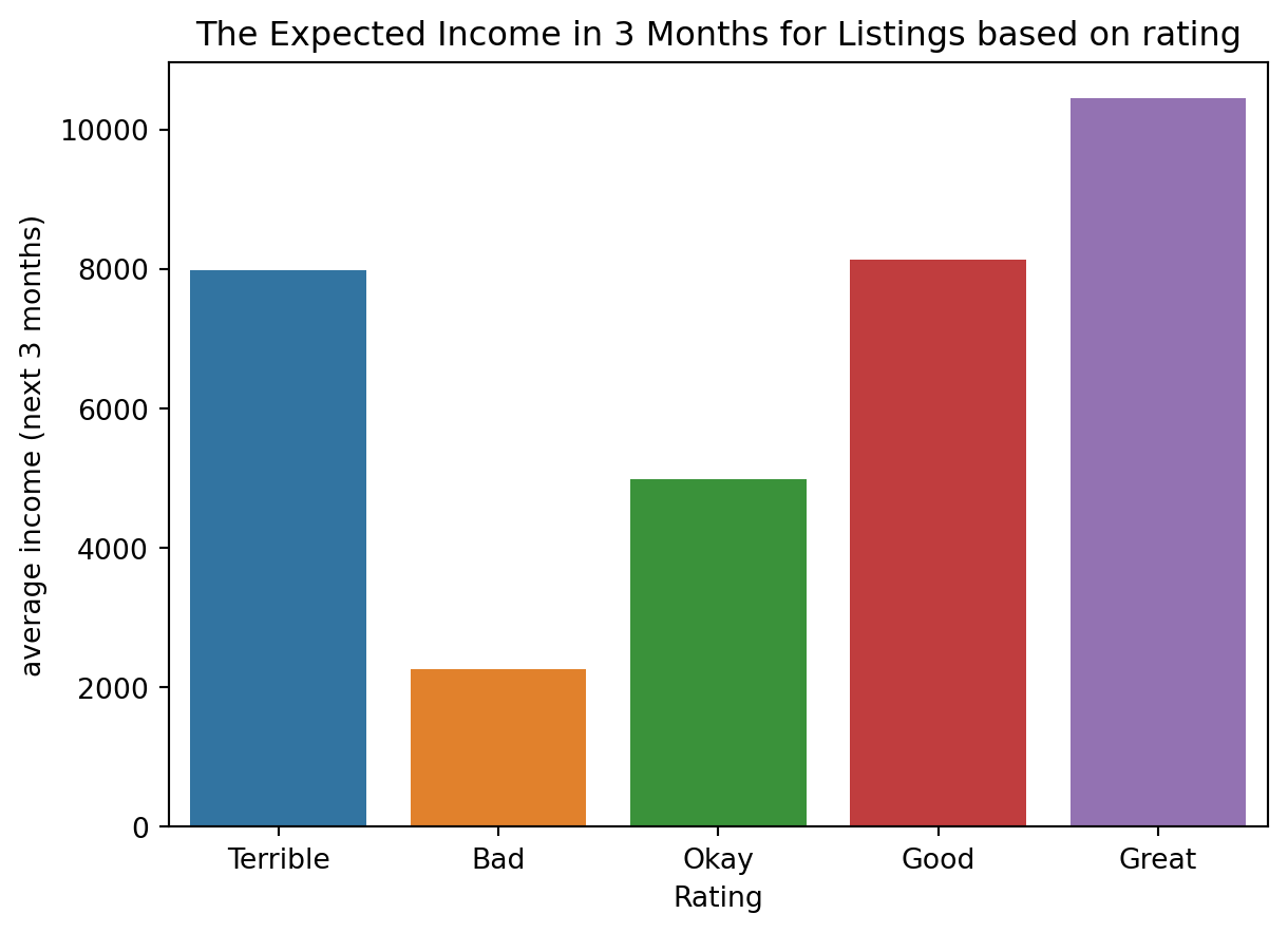
Does the Location Rating effect the expected average income (next 3 months)

Code

data = romeListings.groupby("rating_location_category")["expected_income_coming_3m"].mean().sort_values(ascending=False)
sns.barplot(x=data.index, y=data)
plt.title("The Expected Income in 3 Months for Listings based on rating")
plt.xlabel("Rating")
plt.ylabel("average income (next 3 months)")
plt.show()

Frome the above figure, it looks like listings with Great location review score are expected to have the highest minimum income for the next three months.

Code

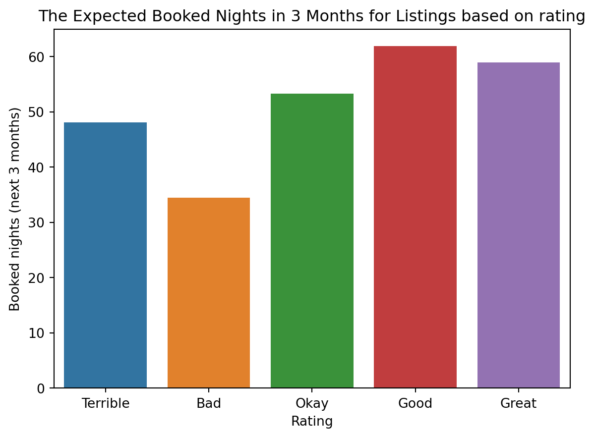
data = romeListings.groupby("rating_location_category")["expected_booked_nights_coming_3m"].mean().sort_values(ascending=False)
sns.barplot(x=data.index, y=data)
plt.title("The Expected Booked Nights in 3 Months for Listings based on rating")
plt.xlabel("Rating")
plt.ylabel("Booked nights (next 3 months)")
plt.show()

It seems that listings with Great, Good or Okay location review score are expected to be booked more than the other categories for the next three months.

What (Bedrooms, Room Type) combination have highest expected income average for the next 3 months?

Code

nBookedNightinNigh=romeListings.groupby(["room_type","bedrooms"])["expected_income_coming_3m"].agg(["mean","count"])
temp=nBookedNightinNigh[nBookedNightinNigh["count"]>11]["mean"].sort_values(ascending=False).head(5)
fig = px.bar(x = list(map(str,list(temp.keys()))), y = temp.values, title = "The highest Expected Income average of listings for every (Bedrooms, Room Type) combination", labels={
    "y": "average income (next 3 months)",
    "x": "(Bedrooms, Room Type)"
})
fig.show()

Listings that are an entire home or an apartment seems to be expected to have the highest income average for the next three months, and an entire home or an apartment with seven bedrooms are expected to have the highest income average with 65.5K

What (Bedrooms, Room Type) combination have highest minimum income average for the past 12 months?

Code

nBookedNightinNigh=romeListings.groupby(["room_type","bedrooms"])["min_income_past_12m"].agg(["mean","count"])
temp=nBookedNightinNigh[nBookedNightinNigh["count"]>11]["mean"].sort_values(ascending=False).head(5)
fig = px.bar(x = list(map(str,list(temp.keys()))), y = temp.values, title = "The highest income average of listings for every (Room Type, Number of Bedrooms) combination", labels={
    "y": "average minimum income of listings (past 12 months)",
    "x": "(Room Type, Number of Bedrooms)"
})
fig.show()

From the above figure, it seems for the past year, listings that are an entire home or an apartment also have the highest income average for the past year, and an entire home or an apartment with seven bedrooms have the highest income average with 7.8K.

Code

data = romeListings.groupby("bedrooms")["expected_income_coming_3m"].agg(["mean", "count"])
data = data[data["count"]>11]["mean"].sort_values(ascending=False).head(10)
fig = px.bar(x = data.index, y = data, title = "The highest Expected Income average of listings for every Bedrooms count", labels={
    "y": "average income (next 3 months)",
    "x": "Number of Bedrooms"
})
fig.show()

We can see that listings with seven bedrooms are expected to have the highest average income for the next three months, followed by 8, 6 and 5 bedrooms.

Conclusion

To increase the profitabilty of your invesment in Rome:

• Have a verification mark.
• Have a profile picture.
• Invest in the top neighbourhood: ‘II Centro Storico’.
• Invest in the room type: Entire Home/Apt in ‘II Centro Storico’, with 7 bedrooms
• Try not to exceed the average prices, might lead to bad Scores Value.
• Try to response as quick as possible.
• Provide an instant booking.
• Include the following amenities: WiFi, Hair Dryer, …

Challenges

In this project we faced some challenges, here is some of them:

• Choosing a dataset based on cities.
• A dataset with more than 70 columns, is not easy.
• Cleaning the amenities column, into discrete values.
• First time to use world map library.
• Language and namings difficulties.
• Estimating occupancy and income.

Sources

• http://insideairbnb.com/get-the-data/
• http://insideairbnb.com/rome
• https://python-visualization.github.io/folium/